aimfast
An Astronomical Image Fidelity Assessment Tool
Introduction
Image fidelity is a measure of the accuracy of the reconstructed sky brightness distribution. A related metric, dynamic range, is a measure of the degree to which imaging artifacts around strong sources are suppressed, which in turn implies a higher fidelity of the on-source reconstruction. Moreover, the choice of image reconstruction algorithm and source finder also affects the estimate on-source brightness distribution.
Fidelity Matrices
Image dynamic range
Dynamic range is a measure of the degree to which imaging artifacts around strong sources are suppressed, which in turn implies a higher fidelity of the on-source reconstruction. Here we determine it in three ways: Obtaining the quotient of - highest peak flux (\(flux_{peak}\)) and the absolute of the minimum flux (\(flux_{min}\)) around the peak in the residual image. - highest peak flux (\(flux_{peak}\)) and the rms flux (\(flux_{local_rms}\)) around the peak in the residual image. - highest peak flux (\(flux_{peak}\)) and the rms flux (\(flux_{grobal_rms}\)) in the residual image.
Statistical moments of distribution
The mean and the variance provide information on the location (general value of the residual flux) and variability (spread, dispersion) of a set of numbers, and by doing so, provide some information on the appearance of the distribution of residual flux in the residual image. The mean and variance are calculated as follows respectively
and
whereby
The third and fourth moments are the skewness and kurtosis respectively. The skewness is the measure of the symmetry of the shape and kurtosis is a measure of the flatness or peakness of a distribution. This moments are used to characterize the residual flux after performing calibration and imaging, therefore for ungrouped data, the r-th moment is calculated as follows:
The coefficient of skewness, the 3-rd moment, is obtained by
If there is a long tail in the positive direction, skewness will be positive, while if there is a long tail in the negative direction, skewness will be negative.

Figure 1. Skewness of a distribution.
The coefficient kurtosis, the 4-th moment, is obtained by
Smaller values (in magnitude) indicate a flatter, more uniform distribution.
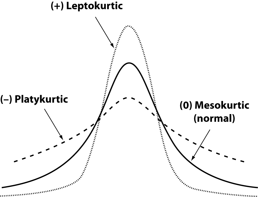
Figure 2. Kurtosis of a distribution.
Furthermore, there is median absolute deviation which is a measure of how distributed is the residual data with regards to the median. This can be compared with the standard deviation to verify that the residuals are noise-like (and Gaussian).
Installation
Installation from source, working directory where source is checked out
$ pip install .
This package is available on PYPI, allowing
$ pip install aimfast
Command line usage
Get the statistics of the residual image
$ aimfast --residual-image cube.residual.fits
Get the residual image stats and dynamic range in one step where argument -af is a factor to multiply the beam area to get target peak area:
$ aimfast --residual-image cube.residual.fits --restored-image cube.image.fits -af 5
or using sky model file (e.g. tigger lsm.html):
$ aimfast --residual-image cube.residual.fits --tigger-model model.lsm.html -af 5
NB: Outputs will be printed on the terminal and dumped into fidelity_results.json file. Moreover if the source file names are distinct the output results will be appended to the same json file.
$ cat fidelity_results.json
$ {"cube.residual.fits": {"SKEW": 0.124, "KURT": 3.825, "STDDev": 5.5e-05,
                          "MEAN": 4.747e-07, "MAD": 5e-05},
       "cube.image.fits": {"DR": 35.39, "deepest_negative": 10.48,
                           "local_rms": 30.09, "global_rms": 35.39}}
Additionally, normality testing of the residual image can be performed using the D’Agostino (normaltest) and Shapiro-Wilk (shapiro) analysis, which returns a tuple result, e.g {‘NORM’: (123.3, 0.1)}, with the z-score and p-value respectively.
$ aimfast --residual-image cube.residual.fits --normality-model normaltest
Furthermore, a comparison of residual images can be performed as follows: To get random residual flux measurements in residual1.fits and residual2.fits images
$ aimfast --compare-residuals residual1.fits residual2.fits --area-factor 2 -dp 100
where –area-factor is the number to multiply the beam size to get area and -dp is the number of data points to sample. In case the beam information is missing from the image header use –psf-image | -psf, the point spread function file or psf size in arcsec, otherwise a default of 5 arcsec will be used. To get on source residual flux measurements in a residual1.fits and residual2.fits images
$ aimfast --compare-residuals residual1.fits residual2.fits --tigger-model model.lsm.html
where –tigger-model is the name of the model or catalog file to locate exact source residuals. For random or on source residual noise comparisons, the plot on the left shows the residuals on image 1 and image 2 overlayed and the plot on the right shows the ratios. The colorbar shows the distance of the sources from the phase centre.
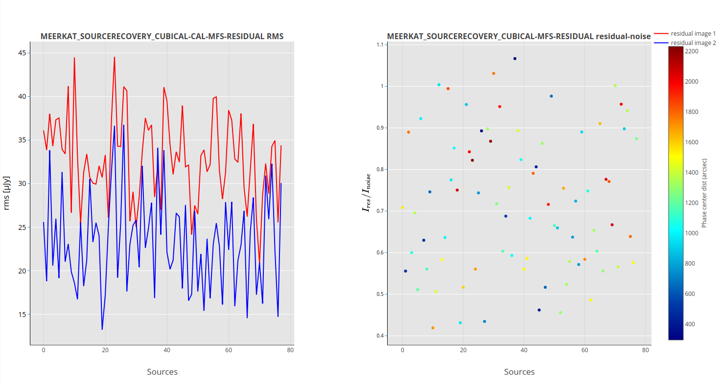
Figure 3. The random/source residual-to-residual/noise ratio measurements
Moreover aimfast allows you to swiftly compare two (input-output) model catalogs. Currently source flux density and astrometry are examined. It returns an interactive html correlation plots, from which a .png file can be easily downloaded.
$ aimfast --compare-models model1.lsm.html model2.lsm.html -tol 5
where -tol is the tolerance to cross-match sources in arcsec. Moreover -as flag can be used to compare all source irrespective of shape (otherwise only point-like source with maj<2” are used). Access to (sumss, nvss,) online catalogs is also provided, to allow comparison of local catalogs to remote catalogs.
$ aimfast --compare-online model1.lsm.html --online-catalog nvss -tol 5
In the case where fits images are compared, aimfast can pre-install source finder of choice (pybdsf, aegean,) to generate a catalogs which are in turn compared:
$ aimfast --compare-images image1.fits image1.fits --source-finder pybdsf -tol 5
After the first run attempt one of the outputs is source_finder.yml file, which provide all the possible parameters of the source finders. Otherwise this file can be generated and edited prior to the comparison:
$ aimfast -gd my-source-finder.yml
$ aimfast --compare-images image1.fits image2.fits --config my-source-finder.yml -sf pybdsf -tol 5
For Flux density, the more the data points rest on the y=x (or I_out=I_in), the more correlated the two models are.
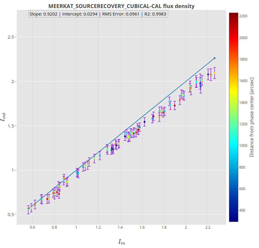
Figure 4. Input-Output Flux model comparison
For astrometry, the more sources lie on the y=0 (Delta-position axis) in the left plot and the more points with 1 sigma (blue circle) the more accurate the output source positions.
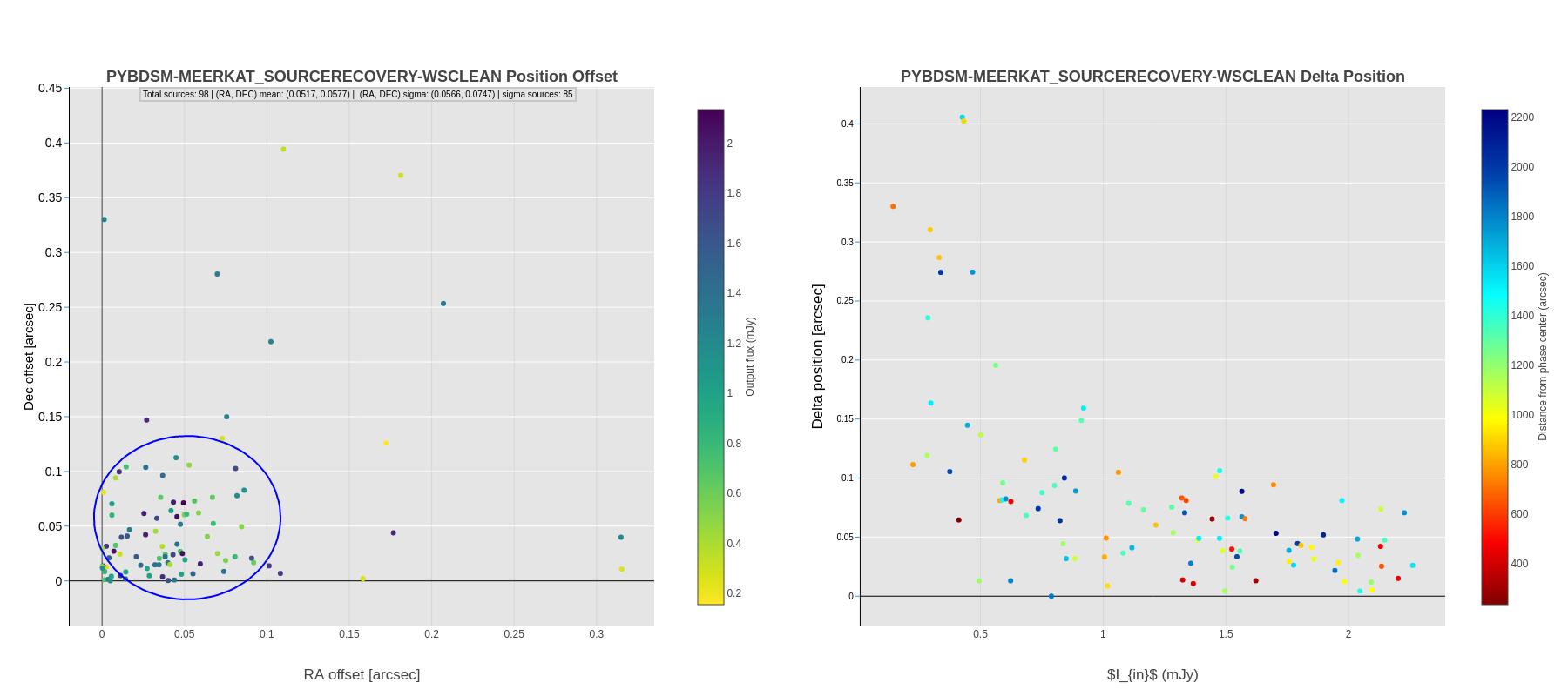
Figure 5. Input-Output Astrometry model comparison
Lastly, if you want to run any of the available source finders, generate the config file and edit then run:
$ aimfast -gd my-source-finder.yml
$ aimfast source-finder -c my-source-finder.yml -sf pybdsf